Difference between AS-WAS and AS-IS reporting in a Data Warehouse

Every DWH/ETL developer should be well versed about this concept, I was a couple of days back explaining the same to a person new in our team. That's when it struck me, why not a post on the same, so here goes. I will try to explain the same, giving an example.

Imagine a customer making monthly payments to a bank loan each month from January 2020 till May 2020, where at the end of the month of March, he changed his Address, he moved to a new county/district. This information will be captured in Customer dimension in EDW as below,

So you have your first customer record, which expires on 31st March, and a new record,which is currently active from 1st April 2020 till high end date.

Now imagine we have a transaction table as below with the 5 payment transactions as discussed before from January 2020 till May 2020, so customer has made 3 payments at his first address and the rest 2 at his new address.

Let us discuss now the AS-IS and AS-WAS concepts with this dataset, most EDW/Reporting systems use "AS-WAS" concept for grouping, as per this, suppose you are grouping the payment amount based on DISTRICT column in "AS-WAS", the result set would look as below,

So as you can infer from the result set above, in AS-WAS grouping, the snapshot as of Transaction date gets reported, i.e when T1, T2 and T3 payments were made, the customer was at Trivandrum, and later when T4 and T5 payments were made, he moved to Cochin.

However in "AS-IS" reporting, all payments are reported against the current active record of the customer, hence the full amount will be reported against Cochin in this case, see result set below to understand,

In AS-IS reporting, the measures reported against dimension attributes as of current date.

Dimensional Modelling - Loan Dimension in Banking Data warehouse - Part 1

Loan Dimension in a Banking Enterprise Data warehouse is very crucial. It is undoubtedly one of the if not biggest data warehouse dimension in a banking DW architecture. It is also of one of the most confirmed dimensions in an banking data warehouse. Loan dimension has a lot of textual attributes and also an almost equal number of measurable attributes. It is also joined to many other entities of a banking EDW. A few examples of the key entities are the following,

• Branch 
• Primary Customer
• Teller
• Loan Product
• Time/Dates ( Maturity, Commencement, Settlement, Disbursement, Dormancy )

As we discussed before there are many textual attributes are unique to a loan dimension and few examples are listed below,

Account status,
Product Name
Settlement, Account open date, Loan Approved date, First disbursement date, Last Transaction date.

Considering the size of a loan dimension it can be split into multiple tables to improve performance and maintainability. A good way to start modelling a dimensional model is to create bus matrix as suggested by Ralph Kimball.

The bus matrix for a Loan dimension in an ideal scenario would look as below,

Bus Matrix for Loan Dimension.

The loan dimension being one of the largest entities will take up a number of columns. It is a good practice to split the dimension as follows in case it has a large number of table,

The first partition of the dimension table should have all the most commonly used attributes, like Status, Balance etc. The second partition should have all the measurable attributes like Approved amount, applied amount, and the corresponding date keys. These measures can also act as attributes in some cases. The second table can also be used as a fact in some cases. The third or the next partitions should have all the junk values related to the dimension. Advised to put all the rarely used dimension columns here. These tables can be made to one single dimension in BI tool for example with the help of Logical table sources in OBIEE.

Why we are advising this strategy is because otherwise the maintenance of this table would be down the line a headache. Imagine a table with 500 columns. A single insert statement would be of large size. Hence taking more time to execute and load into target schema.

Naming conventions, You can go ahead with standard naming conventions followed by Oracle or have one of your own. An Oracle naming standard would be,

W_LOAN_D

If you have multiple sources, Then you can have a source abbreviation also in the same name.

Data warehouse basics: What is Incremental Data Load ?

So we are back again to brush the basics. I have always felt that for a BI/DW developer to become successful he/she should have a very strong base about the basics. Here is one basic concept we hear often, Incremental load.

So what exactly is Incremental data load ?

Incremental data load is a type of data load scenario in a Data warehouse environment where the data that is updated/new are inserted to the target data warehouse with each scheduled run.

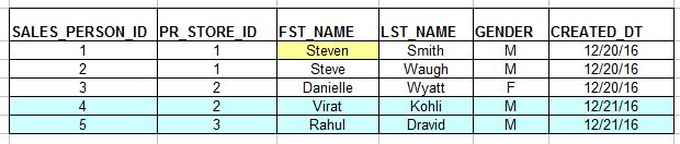
Imagine a sales person table as below which will be our source table in this case.

On the first day of loading to an EDW table, all the above three records would be moved.  The target table would be same as above. 

Now a day after they have added two new employees and also made a change to first name of a previous employee. Refer the screenshot below, 

Here with incremental update the two new records are considered and written to the target table. Also checks the source if the already existing records in EDW has any changes in source. There is the first record where FST_NAME was changed from Steve to Steven, hence this record is also considered and the change is updated in the target table. 

The advantages of incremental loads are the following,

1. Reduces a major chunk I/O operations between source and target. 
2. Faster than a full base load.

Indexing Strategy in DW: What are Indexes, Types and Significance ?

We are starting off a new series on Indexing strategies in an Oracle Data warehouse. Before going into detail let us first see what an Oracle Index is. 

A database index is a database object that is created to optimize the performance of a read/select statement on a particular table. They greatly reduce the I/O operations on a table by reducing the rows processed. 

Oracle defines Indexes as below, 

An index is an optional structure, associated with a table or table cluster, that can sometimes speed data access. By creating an index on one or more columns of a table, you gain the ability in some cases to retrieve a small set of randomly distributed rows from the table. Indexes are one of many means of reducing disk I/O.

'Indexing' is a term coined for the strategy used for indexing in a particular relational DBMS. Let us see the advantages of indexing

1. Avoid full table scans and there by reducing the cost and time to retrieve from a database table.
2. They avoid sorting of oracle queries. which in turn reduces the time for retrieval of data. 

There are different kinds of Indexes available in Oracle and they are the following, 

• B-Tree or Normal Indexes
• Bitmap indexes
• Function based indexes

B-Tree Indexes are the most common indexes in oracle database. by default a B-Tree index is generated. Here values are stored as leafs. There are branch blocks and leaf blocks. Branch blocks contain the leaf blocks where actual pointer values are stored. Here one entry in an index points to one row.

Bitmap indexes are usually created for low carnality columns like Gender, flags etc. In Bitmap indexes one index entry points to multiple rows. 

Function based indexes are indexes created on columns with a function. If one was to apply calculations on a particular column then function based indexes are created on that particular column.